Exposure modelling in IEHIAS
- The text on this page is taken from an equivalent page of the IEHIAS-project.
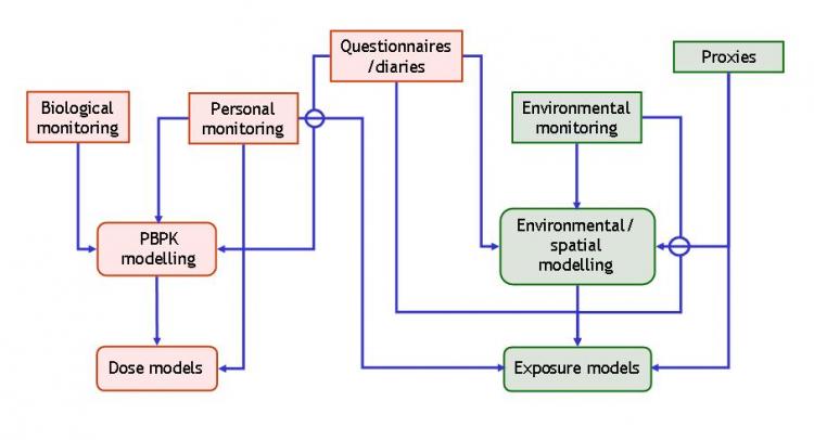
Exposure assessment is an important part of any intregated environmental health impact assessment, and also often one of the most demanding. Difficulties come from the need to estimate exposures of large numbers of people at a spatial and temporal resolution that does not mask or distort important variations in exposure - and to do so in the context of a highly mobile and variable population and inadequate environonmental and demographic data. In the face of these challenges, a wide range of methods of exposure assessment have been devised, and often several of these need to be used in combination in order to provide a reliable basis for impact assessment (Figure 1).
Contents
Methods of exposure assessment
As Figure 1 shows, exposure assessment can be done via two main approaches: monitoring and modelling. Each of these, however, may be applied in two different ways - either targetted at humans themselves (anthropic methods) or at the context within which exposure occurs (environmental methods).
These methods are not independent of each other. Monitoring data, for example, are generally required as inputs to models and to validate model results. Modelling is often needed to extrapolate from sample measurements to the wider population - and, in the context of most health impact assessments, to predict exposures for scenarios that have not yet occurred. Environmental methods are often required to provide context to biological (PBPK or dose) models, while anthropic models are used to help interpret results obtained from environmental approaches.
The different methods nevertheless differ considerably in their specific strengths and weaknesses, and in their adaptability to different situations. In general, direct measurements of humans (e.g. biomonitoring and personal exposure monitoring) can be assumed to provide the most accurate estimates of the subject’s true exposure, and are often used as the standard against which other methods are validated. Likewise, models targetted at biological and biochemical processes (e.g. PBPK and dose models) should provide greater accuracy than environmental models, which are inherantly further removed from the exposure experience. Limitations of data and knowledge, however, often inhibit the use of these approaches, with the consequence that exposure assessment has to resort to less direct, environmentally-based methods.
Whatever approach is taken, it is important to remember that exposures do not just depend on the nature of the agent and its behaviour or distribution in the environment. It depends fundamentally also on the behavioural and other characteristics of the people concerned, such as their time activity patterns, diet and physiology, all of which help to determine where, when, how and for how long individuals become exposed. For this reason, personal data derived from questionnaires or diaries (or in the absence of these, from popualtion level surveys such as national censuses) are usually important, and feed into most methods of exposure assesment at some stage.
As this also implies, exposure assessment often involves combining data and methods from different levels - e.g. at individual, micro-environmental, neighbourhood and national or population scales. While using broader-scale data in the assessment may mean that the specificity of individual experience is lost, the analysis becomes more generally applicable, and enables exposure distributions for the whole population (or population grouups) to be assessed. These distributions can then be used to create specific exposure scenarios withjin which to analyse the impacts of different policy actions (Ott et al. 2006).
Figure 1. Methods for exposure assessment
Key: Rectangular boxes = monitoring; bevelled boxes = modcelling; red = biological methods; green = environmental methods
Exposure modelling
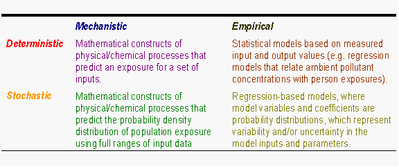
Exposure models (like other models) can loosely be classified into four categories, as listed in Table 1. In principle, mechanistic models are likely to be more robust, in that they are based on some understanding of the underlying processes that affect exposure; they should therefore translate with reasonable reliability between different data sets or situations. Often, however, they do not give the best possible level of prediction in specific contexts, because they have not been attuned to the specific data. They are also, of course, dependent on the level of real understanding of the processes involved. In many situations, therefore, empirical approaches (often based on regression analysis) are used instead. These carry two crucial dangers: while they may fit the data well (and thus appear to give good estimation of exposures in terms of the β-coefficient or regression r2 of the models), they may not be realistic; and while they may work well (and be valid) in the conditions under which they were initially developed, they may be unreliable when applied in different situations. Empirical models therefore should always be revalidated (and may need to be recalibrated) when used outside the range of the original data.
Deterministic methods are often preferred by users, because they are easier to apply and appear to give explicit answers. They ignore, however, the uncertainties that are inherent in the modelling and the variability that occurs in the real world. They can therefore be misleading and may suppress valuable debate about policy options and falsely restrict policy choices. Probabilistic models, in contrast, are designed to reflect these uncertainties and thereby present results in terms not of fixed estimates but of exposure distributions. While this may seem to leave decision-makers without a clear message, it is a more honest reflection both of the status of the science and of the way the real world operates. For policy assessments, therefore, mechanistic-stochastic models are likely to be the most informative.
Table 1. The categories of exposure models (WHO 2005)
Population modelling
Population data play a range of vital roles in integrated assessment of environmental risks to health:
- As proxies for source activity and intensity data in models of emissions or environmental concentrations (e.g. in terms of domestic waste production, traffic density, atmospheric emissions, air pollutant concentrations)
- As a basis for modelling and estimating population exposures (e.g. by intersection of population data with environmental data, by extrapolation from personal monitoring or biomonitoring data)
- As a source of information on vulnerability (e.g. related to age, sex or socio-economic status).Population density and composition are both highly variable, often over short distances.
Substantial changes in population can also occur over periods of a few years not only as a result of natural changes of birth and death but also through migration and urban development. The spatial and temporal resolution of these data is therefore often critical in determining their utility for healtjh impact assessment. While some assessments can cope with aggregated data, based for example on national decennial population counts, for many purposes the data need to be available at the resolution of 1 km or less, in order to reflect local variations in environmental conditions, and for time periods of no greater than one or two years. Additionally, for many applications data are needed not as totals for the whole population, but for specific population groups, defined in terms of age, sex, ethnic origin etc. The ability to provide data at these levels of detail (i.e. cross-stratified by area, year, and population group) is likely to be one of the main limiting factors in the utility of available population data.
Two forms of population modelling are therefore likely to be necessary in many integrated assessments:
- temporal modelling (population projections), to calculate likely changes in population numbers and structure for future years, under the various policy scenarios being assessed;
- spatial modelling, to estimate the local distribution of these population groups under the various scenarios.
Population projections
Population projections are an estimate of a future population. Unlike censuses, in which information about the members of the population is systematically collected and recorded, population projections typically involve mathematical models based on pre-existing data. The projections are actually scenarios based on assumptions about the factors which influence population changes, such as fertility, mortality and migration. Projections of this type are often needed in assessments, for example, to indicate the size (and susceptibility) of the population for future years, to compute rates and DALYs for health outcomes with long lag periods (e.g. some cancers), and to take account of changes in population distribution and structure caused by the policy or other factors being analysed.
Estimates and projections for population size, growth and structure are available from various sources including the United Nations (world), Eurostat (for Europe) and national statistics offices. Depending on the data provider, projections may be available as world-wide, regional, national or sub-national estimates and include sex and/or age breakdown. The typical time horizon is the mid 21st century, but long-range projections to 2150 and 2300 are also available from, for example, the United Nations (UN 2004).
Regional (NUTS 3) projections to the year 2030 are currently available from Eurostat for European Member States. For some countries, more detailed projections may be obtained through the national statistics office. For example, the “2008-based Subnational Population Projections for England” (ONS 2010) provides local authority level estimates with age and sex breakdown to the year 2033. These are trend based projections, meaning that assumptions for future levels of births, deaths and migration are based on observed levels over the previous five years (2004 to 2008). The projections thus show what the population structure will be assuming the recent trends continue.
Spatial population modelling
Reliable information on the location and distribution of the population is essential for risk assessment in order to differentiate between, and calculate, population-level exposures. Census data provide routinely available information on population numbers and composition, generally on a decennial basis. By their design, however, census tracts - arranged to facilitate enumeration rather than to reflect the underlying geographic distributions of population - are of limited value for exposure assessment.
Census tracts are rarely uniform in size or population numbers, and typically cover large geographic areas including unpopulated lands (e.g. rural land, parks and industrial developments). The smallest geographic unit for the EU administrative regions, for example, is the Local Administrative Unit 2. Outside densely built-up urban centres most LAU2 regions are around 5-10 km2. In rural areas, they may be in excess of 100km2. Where the LAU2 regions are this large, the population tends to be dispersed or clustered in small towns with inhabitants typically residing in only a small proportion of the region.
In response to these problems, several spatial disaggregation methods have emerged to estimate small-area population for various science and policy applications including risk assessment. The methods range in complexity from simple area weighting (Goodchild and Lam1980) to dasymetric mapping techniques (Briggs et al. 2007; Flowerdew and Green 1994; Harris and Longley 2000; Mennis 2003).
Area weighting, for example, is used to construct the gridded population of the world (GPW-3) database (CIESIN 2004). It is an approximate approach, however, which relies on the (often false) assumption that the population is evenly distributed within each census district. To develop more reliable models of population distribution requires more sophisticated techniques incorporating additional data on exogenous variables that can be assumed to reflect lower level (i.e. within census tract) variations in population density. These more complex dasymetric mapping or disaggregation techniques often use land cover data derived from satellite imagery to provide the necessary ancillary information for modelling.
Exposure factors
Exposures to (and intake of) environmental contaminants depends to a large degree on the characteristics of the people concerned. These comprise not just their physical characteristics, such as height and weight, which influence the bodily area available for exposure and the mass into which the contaminant can be absorbed, but also the many different aspects of behaviour that help to determine opportunities for exposure and efficiency of intake. These latter factors involve almost every aspect of lifestyle - e.g. diet, exercise, transport choices, home environment, dress, smoking and patterns of socialisation - and all the many different elements of social and personal context and history that in turn influence these (e.g. age, gender, income, culture).
If exposure and intake assessment are to be reliable, and properly reflect the variations in exposure likely to occur within a study population, they need to take account of these personal and social influences. This is all the more important in integrated environmental health impact assessments, where concern is often about how exposures will change under different policy scenarios. These changes are not just a function of changes in the environment; they occur also because of associated changes in behaviour. Policies aimed at reducing urban air pollution, for example, are often targetted at changing emissions from transport systems and housing. Achieving either of these almost inevitably involves adaptations in behaviour, both as a deliberate part of the policy itself (e.g. by encouraging a shift from private to public transport, or installation of insultaion in the home) and as a concomittant or incidental response. Even a simple switch from car to bus or train for the journey to work, for example, may result in a change in travel routes, travel time, journey duration, amount of time spent outdoors and even style of dress, all of which may affect exposure and intake of pollutants and may modify the overall health impact of the policy. Moreover, many of the behavioural and lifestyle characteristics that modulate exposures and intake in these ways are associated with gender, socio-economic status or ethnicity, and are thus the potential source of social inequalities in risk and so-called environmental injustices. For this reason, too, they need to be considered in assessments.
Allowing for these effects in any detailed way is difficult, especially in large population studies, where individual level data on time activity, lifestyle and personal characteristics is likely to be sparse. Because of their social and demographic associations, however, they can be approximated with some degree of confidence at group level - e.g. stratified by age, gender, socio-economic status or occupation. Behavioural, lifestyle, social and personal data are all extensively collected, for exampe, both as part of national censuses and more targetted social surveys. Several attempts have also been made to bring together relevant information in the form of databases on exposure factors. These provide statistics on a wide variety of behaviours and other contextual factors likely to affect exposures. They can best be used in exposure assessments either deterministically, to adjust estimates of 'average exposure' for specific population sub-groups, or probabilistically to represent the distribution of exposures likely to occur within a group as a consequence of behavioural, lifestyle and personal influences.
Consumer products exposure models
Models for exposure to consumer products (including pesticides, personal care products, cleaning products, etc.) must usually account for multiple exposure pathways. Dermal contact and ingestion - particularly non-dietary ingestion - are important routes of exposure. Inhalation may also be considered. These models may vary greatly in their approach to modeling exposure or intake/dose.
Scope
Purpose:
Models of exposure to consumer products are needed to provide estimates of potential risks arising from contact with, and use of, everyday household articles and materials.
Boundaries:
The main limitations are:
- Ingestion and dermal contact rates are very heterogeneous within and across populations - quantification of this information is time- and resource-intensive, so data are not widely available. Rates in children and workers tend to be better studied than in other populations.
- Transfer coefficients and absorption rates are not well quantified for many substances. QSAR has been used in some cases, but the relationships have not been established as robust yet.
Method description
Input:
- Source emissions
- Time-activity patterns for the population of interest (e.g. children, elderly, adults, etc.)
- Contact times and behaviour
- Intake rates
- Transfer coefficients
- Physiological parameters (if dose is of interest)
Output:
- Absorbed dose
- Intake
- Exposure concentration
Rationale:
Consumer product models may calculate exposure or intake. Intake is most likely if the exposure routes are ingestion or dermal uptake.
Exposure = Σ(concentration (= dilution x temporal decay x removal x medium transfer) x contact time/rate)
or
Intake = Σ(concentration (= dilution x temporal decay x removal x medium transfer) x intake rate)
Models account for exposure or intake during specific use scenarios, and may treat multiple pathway exposure either in sum or separately. Default source values and parameters are possible in some models if the user does not have further information.
Method:
Consumer products exposure models can be deterministic or stochastic in approach.
Generally, several scenarios may be investigated by a model. These scenarios involve different applications of a product. The product distribution in the environment and contact media is modelled or derived from measured concentrations and subsequent contact frequency and duration data are used to calculate exposure. Inhalation applications may or may not include inhalation rates, while intake is calculated for ingestion and dermal exposure. Some models may also include dosimetry calculations.
Time micro-environment activity modelling
Exposure timelines
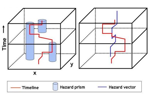
Human exposure and intake of environmental contaminants requires that people spend time in contact with the agent. This may occur in different places, in different settings (micro-environments), at different times and for different durations. The level of exposure thus depends on where people are, when, and for how long, and conditions at those locations during those times. Over a period of time (e.g. a lifetime) people may also be exposed to a range of pollutants, to varying degrees, and more-or-less repeatedly. Exposure is rarely, therefore, a one-off event, but more commonly an extended process or experience (Figure 1, below). In terms of health effects, likewise, concern is not only about the instantaneous or acute implications of short-term exposures, but also about the effects of cumulative exposures and chronic effects.
Figure 1. Timelines and exposure to environmental hazards
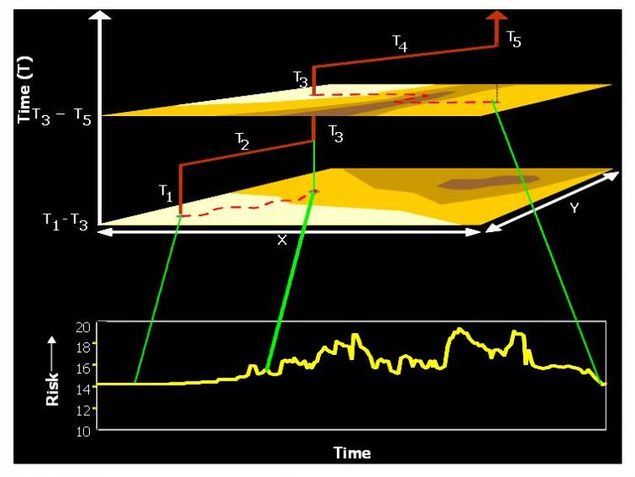
For these reasons, exposure is not determined only by the environmental fate of a pollutant (i.e. what happens to it after release) nor the distribution of the pollution in the environment. It depends, equally, on human time-activity patterns within this changing pollution field (Figure 2). It is influenced, therefore, by all the factors that influence people's behaviour: their age, gender, socio-economic status, cultural context and adopted lifestyle, along with individual physiology (e.g. height and weight). Ideally, all these determinants need to be considered in assessing exposure and intake as part of impact assessments. The extent to which this is possible, however, inevitably depends on the context within which the assessment is done. Constraints of data, knowledge, computer resources, finance and time inevitably mean that not every factor can usually be taken into account. The art of exposure assessment is thus to achieve the most reliable possible estimates within these constraints.
Figure 2. Time activity and the exposure profile
Time-micro-environmental activity modelling
Time micro-environment activity (TMA) models provide a means of estimating exposures in relation to the activity timelines. They combine concentrations in specific locations (micro-environments) and data on the locations, the time spent in these locations, and in some situations the activities that individuals perform in these locations.
Micro-environments are defined as a space in which contaminant concentration can be considered to be spatially uniform during some specific interval (typically a room, car, back yard, etc.). These models represent total personal exposure, and are used mainly for inhalation exposures. Concentration inputs to TMA models come from measured data or other models, such as dispersion models. Some TMA models also have the ability to calculate intake and dose using physiologically based pharmacokinetic (PBPK) models.
Input
- Probabilistic models require inputs (thgough not necessarily all) to be in the form of distributions
- Micro-environmental concentration distributions (e.g. inside homes, in workplaces, in vehicles, etc.)
- Time-activity patterns for the population of interest (e.g. children, elderly, adults, etc.)
- Contact times
- Inhalation rates
- Physiological parameters (if dose is of interest)
Output
- Personal exposure or intake concentrations for individuals and populations over a specified period of time
- Outcomes can be in distributional form
Rationale
The major benefit in comparison with models of the ambient environment is that the effect of spending time in different exposure settings (e.g. indoors and in traffic) can be separately accounted for. The role of these special micro-environments depends on the type of pollutants studied, and on the extent to which concentrations in the micro-environments differ from surrounding external environment. This depends on a range of factors, including the presence of local emission sources within the micro-environment, and the porosity of the boundary between this and the external environment. Concentrations of traffic-derived particulates, for example, are usually less in indoor air than in ambient environments, because of restricted air exchange and penetration of particulates. On the other hand, indoor concentrations of other pollutants may be substantially increased compared to outside because of the presence of indoor sources (e.g. smoking, heating, cooking). Similarly, ratos of air pollution in-vehicle compared to at the roadside vary, depending on ther source, vehicle ventilation conditions (whether windows are open, whether air conditioning is operating) and specific driving conditions (vehicle spacing, speed etc).
Method
TMA models address exposure specifically, including the time spent in contact with the contaminated medium across a specified exposure time.
Exposure = time-weighted average exposure over micro-environments visited
or
Exposure = Σ(concentration (= dilution x temporal decay x removal x medium transfer) x contact time/rate)
Exposure is thus estimated as the concentration to which an individual comes into contact within a particular micro-environment multiplied by the fraction of total time (over a time frame of interest, be it a lifetime or a shorter period) spent in the micro-environment.
For models that can calculate dose, absorption coefficients and partition coefficients for the different physiological compartments also have to be incorporated.
The micro-environment model uses average concentrations experienced and times spent in each micro-environment as inputs. These are typically described as probability density distributions of the average concentrations, and times spent in the same micro-environments, usually derived from time-activity diaries. Concentration data can be obtained from measurements or by modelling. In the case of indoor air, for example:
- Ambient air pollutant concentrations may be derived from measurements at local routine monitoring sites, or by dispersion modelling;
- These can be translated into estimates of indoor concentrations using mass balance/ventilation models;
- Contributions from indoor sources are added using data on the presence/absence of sources, or indoor release/mixing models.
Some TMA models also incorporate two-stage Monte Carlo simulation, thereby allowing for propagation of both variability and uncertainty through the model. In these models, uncertainty distributions for model parameters would need to be included.


