Calibration

This page is a encyclopedia article. The page identifier is Op_en5031
Moderator:Jouni (see all)
This page is a stub. You may improve it into a full page.
Upload data Show results

Calibration and informativeness are measures of expertise. An expert is well calibrated if she is able to correctly predict the probability that her answers actually turn out to be correct. This can be evaluated by observation: if an expert says that she is 80 % sure about the answer, it should mean that when taking ten answers with similar certainty, eventually two of them, on average, should turn out to be incorrect. If the actual result is lower, the expert is said to be overconfident. Calibration is measured against the truth, when it is revealed. Specifically, calibration is a p value for a statistical test about a null hypothesis that an expert is actually calibrated and neither overconfident nor underconfident.

Informativeness measures the spread of a probability distribution. The narrower the distribution, the more informative it is. Informativeness is a relative measure and it is always measured against some other distribution about the same issue.

Calibration

We have asked for each expert’s uncertainty over a number of calibration variables; these variables are chosen to resemble the quantities of interest, and to demonstrate the experts’ ability as probability assessors. An expert states n fixed quantiles of his/her subjective distribution for each of several uncertain quantities. There are n+1 ‘inter- quantile intervals’ into which the actual values may fall.

Let

$p = (p_1, ... , p_{n+1}) (1)$

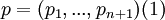
denote the theoretical probability vector associated with these intervals. Thus, if the expert assesses the 5%, 25%, 50%, 75% and 95% quantiles for the uncertain quantities, then n = 5 and p = (5%, 20%, 25%, 25%, 20%, 5%). The expert believes there is 5% probability that the realization falls between his/her 0% and 5% quantiles, a 20% probability that the realization falls between his/her 5% and 25% quantiles, and so on.

Suppose we have such quantile assessments for m seed variables. Let

$s =(s_1, ... , s_{m+1}) (2)$

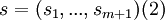
denote the empirical probability vector of relative frequen- cies with which the realizations fall in the interquantile intervals. Thus

s1 = (# realizations less than or equal to the 5% quantile)/m,

s2 = (# realizations strictly above the 5% quantile and less than or equal to the 25% quantile)/m,

s3 = (# realizations strictly above the 25% quantile and less than or equal to the 50% quantile)/m

and, so on.

If the expert is well calibrated, he/she should give intervals such that—in a statistical sense—5% of the realizations of the calibration variables fall into the corresponding 0–5% intervals, 20% fall into the 5–25% intervals, etc.

We may write:

$2mI (s, p)= 2m \Sigma_{i=1}^{m+1} s_i ln(\frac{s_i}{p_i}), (3)$

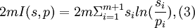
where I(s,p) is the Shannon relative information of s with respect to p. For all s,p with p_i >0, i = 1,...,m+1, we have I(s,p)≥ 0 and I(s,p) = 0 if and only if s = p (see ). Under the hypothesis that the uncertain quantities may be viewed as independent samples from the probability vector p,2mI(s,p) is asymptotically Χ² -distributed with m degrees of freedom: P(2mI(s,p)≤x) ~ Χ²m² where Χ²m is the cumulative distribution function for a Χ² variable with m degrees of freedom. Then

$CAL = 1 - \Chi^2_m (2mI(s,p)) (4)$

is the upper tail probability, and is asymptotically equal to the probability of seeing a disagreement no larger than I(s,p) on n realizations, under the hypothesis that the realizations are drawn independently from p.

CAL is a measure of the expert’s calibration. Low values (near zero) correspond to poor calibration. This arises when the difference between s and p cannot be plausibly explained as the result of mere statistical fluctuation. For example, if m = 10, and we find that 8 of the realizations fall below their respective 5% quantile or above their respective 95% quantile, then we could not plausibly believe that the probability for such events was really 5%. This phenomenon is sometimes called "overconfidence." Similarly, if 8 of the 10 realizations fell below their 50% quantiles, then this would indicate a "median bias." In both cases, the value of CAL would be low. High values of CAL indicate good calibration.

Informativeness

Information is measured as Shannon’s relative informa- tion with respect to a user-selected background measure. The background measure will be taken as the uniform (or loguniform) measure over a finite ‘‘intrinsic range’’ for each variable. For a given uncertain quantity and a given set of expert assessments, the intrinsic range is defined as the smallest interval containing all the experts’ quantiles and the realization, if available, augmented above and below by K%.

The relative information of expert e on a given variable is

$I(e) = \Sigma_{i=1}^{n+1} p_i ln (\frac{p_i}{r_i}), (5)$

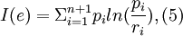
where r_i are the background measures of the corresponding intervals and n the number of quantiles assessed. For each expert, an information score for all variables is obtained by summing the information scores for each variable. This corresponds to the information in the expert’s joint distribution relative to the product of the background measures under the assumption that the expert’s distribu- tions are independent. Roughly speaking, with the uniform background measure, more informative distributions are obtained by choosing quantiles that are closer together, whereas less informative distributions result when the quantiles are farther apart.

Equal-weight and performance-based decision maker

The probability density function for the equal-weight "decision maker" is constructed by assigning equal weight to each expert's density. If E experts have assessed a given set of variables, the weights for each density are 1/E; hence for variable i in this set the decision maker's density is given by

$f_{eqdm,i} = (\frac{1}{E}) \Sigma_{j=1..E} f_{j,i}, (6)$

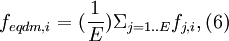
where f_j,i is the density associated with expert j’s assessment for variable i.

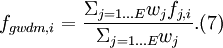
The performance-based ‘‘decision maker’s’’ probability density function is computed as a weighted combina- tion of the individual expert’s densities, where each expert’s weight is based on his/her performance. Two performance-based ‘‘decision makers’’ are supported in the software EXCALIBUR. The ‘‘global weight decision maker’’ is constructed using average information over all calibration variables and, thus, one set of weights for all questions. The ‘‘item weight decision maker’’ is constructed using weights for each question separately, using the experts’ information scores for each specific question, rather than the average information score over all questions.

In this study, the global and items weights do not differ significantly, and we focus on the former, calling it simply ‘‘performance-based decision maker.’’ The performance- based decision maker (Table 4) uses performance-based weights that are defined, per expert, by the product of expert’s calibration score and his/her overall information score on calibration variables, and by an optimization procedure.

For expert j, the same weight is used for all variables assessed. Hence, for variable i the performance-based decision maker’s density is

$f_{gwdm,i} = \frac{\Sigma_{j=1...E} w_j f_{j,i}}{\Sigma_{j=1...E} w_j}. (7)$

The cut-off value for experts that were given zero weight was based on optimising: the cut-off value, a, that gave the highest performance score to the decision maker was selected. The optimising procedure is the following. For each value of a, define a decision maker DMa, which is computed as a weighted linear combination of the experts whose calibration score is greater than or equal to a.DMa is scored with respect to calibration and information. The weight that this DMa would receive if he were added as a ‘‘virtual expert’’ is called the ‘‘virtual weight’’ of DMa. The value of a for which the virtual weight of DMa is the greatest is chosen as the cut-off value for determining which experts to exclude from the combination.

Seed variables

Seed variables fulfil a threefold purpose, namely to enable: (1) the evaluation of each expert’s performance as a probability assessor, (2) the performance-based combina- tion of the experts’ distributions, and (3) assessment of the relative performance of various possible combinations of the experts’ distributions.

To do this, performance on seed variables must be seen as relevant for performance on the variables of interest, at least in the following sense: if one expert gave narrow confidence bands widely missing the true values of the seed variables, while another expert gave similarly narrow confidence bands which frequently included the true values of the seed variables, would these experts be given equal credence regarding the variables of interest? If the answer is affirmative, then the seed variables fall short of their mark. Evidence indicates that performance on ‘almanac items’ (How many heretics were burned at Montsegur in 1244?) does not correlate with performance on variables from the experts’ field of expertise. On the other hand, there is some evidence that performance on seed variables from the field of expertise does predict performance on variables of interest.

Calculations

Informativeness is calculated in the following way for a series of Bernoulli probabilities:

+ Show code- Hide code RInf <- function(s, p) { s*log(s/p) + (1-s)*log((1-s)/(1-p)) }

where s is a vector of actual probabilities and p is a vector of reference probabilities.

Calibration is calculated in the following way:

+ Show code- Hide code 1 - pchisq(sum(2*NQ*RInf(s,p), na.rm = TRUE), nrow(s))

where NQ is a vector of the number of trials for each actual probability.

See also

• Informativeness

Keywords

Expert elicitation, expert judgement, performance

Related files

<mfanonymousfilelist></mfanonymousfilelist>

References

- ↑ 1.0 1.1 1.2 1.3 Jouni T. Tuomisto, Andrew Wilson, John S. Evans, Marko Tainio: Uncertainty in mortality response to airborne fine particulate matter: Combining European air pollution experts. Reliability Engineering and System Safety 93 (2008) 732–744. file in Heande
- ↑ Kullback AS. Information theory and statistics. New York: Wiley; 1959.
- ↑ Cooke R, Mendel M, et al. Calibration and information in expert resolution—a classical approach. Automatica 1988;24(1):87–93.
- ↑ Qing X. Risk analysis for real estate investment. Delft, TU Delft: Department of Architecture; 2002.