Spatial interpolation and extrapolation methods

The text on this page is taken from an equivalent page of the IEHIAS-project.

Environmental measurements are often based on samples, taken at specific locations and in restricted study areas. While these measurements provide useful information about the environmental conditions at or immediately around these locations, they tells us little about the conditions further afield. When wishing to transfer information from past studies to a new area, when needing to estimate conditions at locations not included in the initial survey, or when wanting to produce a contiunuous map of the whole area, therefore, we have to be able to expand from the initial sample sites.

Given what is known as Tobler's ‘first law of geography’ – that things closer together tend to be more alike than things that are far apart – we can often predict conditions at unsampled locations on the basis of information from the nearest available measured points. This process is called spatial interpolation when the predictions are made within the same region represented by the measured points (i.e. within the spatial extent of the measured point locations). Spatial extrapolation is also possible, in which predictions are made outside the spatial extent of the measured points. The difference between spatial interpolation and extrapolation is illustrated in Figure 1, below.

Figure 1. Interpolation and extrapolation

Examples where spatial interpolation or extrapolation may be applied include estimating:

• meteorological conditions such as rainfall or temperature at locations other than weather stations;
• elevation between survey benchmark locations to create a digital elevation model;
• a continuous air pollution surface from a network of regulatory monitoring stations (e.g. measuring NO₂, ozone or particulate matter);
• indicators of water quality (e.g. salinity, temperature, dissolved oxygen) in surface water bodies based on field measurements at a set of sampling locations.

Various methods for interpolation exist in modern geographical information systems (GIS), including (ordered from simple to complex): nearest neighbour, inverse distance weighting, splines, and geostatistical methods such as kriging and co-kriging.

The nearest neighbour method uses Thiessen or Voronoi polygons to define areas of influence around each input (i.e. measured) data point. Thiessen polygons have boundaries that define the area that is closest to each point relative to all other points. This property is mathematically defined by the perpendicular bisectors of the lines between all input data points. In this case, every unsampled location is thus assigned the value of its nearest measurement point.

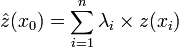
Inverse distance weighting (IDW) combines the notion of proximity with that of gradual change of the trend surface. IDW relies on the assumption that the value at an unsampled location is a distance-weighted average of the values from surrounding data points, within a specified window. The points closest to the prediction location are assumed to have greater influence on the predicted value than those further away, such that the weight attached to each point is an inverse function of its distance from the target location. The general formula is given in Equation 1.

Equation 1

$\hat{z}(s_0) = \sum_{i=1}^N \lambda_i Z(s_i)$

where

Z(s₀) is the value being predicted for the target location s₀

N is the number of measured data points in the search window

λ_i are the weights assigned to each measured point

Z(s_i) is the observed value at location s_i.

Splines are piece-wise polynomial functions that are fitted together to provide a complete, yet complex, representation of the surface between the measurement points. Functions are fitted exactly to a small number of points while, at the same time, ensuring that the joins between different parts of the curve are continuous and have no disjunctions. Splines are often useful for calculating smooth surfaces from a large number of input data points and often produce good results for gently varying surfaces such as elevation. Thin plate splines are a special form of spline, which have particular value in interpolation. These, in effect, replace the exact spline surface with a locally smoothed average which passes as close as possible through the data points. They can be used to remove artifacts (e.g. excessively high or low predicted values) resulting from natural variation and measurement error in the input data.

Unlike the previous methods, geostatistical methods, popularly known as kriging, can estimate both the predicted values and their standard errors. Kriging is an optimal interpolator that uses the spatial configuration and variance of the input data points to determine the interpolation weights and search radii to provide the best, unbiased estimate at unsampled locations. It attempts to divide the spatial variation of a variable into three components: deterministic variation or trend; a random but spatially correlated component (regionalised variable); and uncorrelated noise. It depends on the regionalised variable theory which assumes that the spatially correlated component is homogeneous (i.e. stationary) throughout the surface. The performance of kriging relies on the presence of spatial autocorrelation – meaning that sites which are close together tend to be more similar than those which are further apart.

The nature of the regionalised variable is described by the semivariogram function which is used to optimise the interpolation weights and search radii. The semivariogram is created from the input data points by plotting the semivariance, y(h), against the distance between the pairs of points (h) (Equation 2). For a stationary spatial process, the semivariogram would have a distinctive shape as shown in Figure 2. Different models (e.g. spherical, Gaussian, exponential and linear) can be fitted to the semivariogram and that which gives the best fit chosen for the purpose of prediction.

Equation 2

$\hat{y}(h) = \frac{1}{2n}\sum_{i=1}^{n} [z(x_i) - z(x_i + h)]^2$

where

n is the number of paired observations of the values of attribute z separated by distance h

h is the sample spacing, also called the lag.

Figure 2. General structure and attributes of the semivariogram

At large values of lag (h) the semivariogram tends to level off at the sill. The sill indicates the range beyond which there is no spatial dependence between the input data points. Within the range, spatial autocorrelation exists, so that sites close together have a smaller semivariance. Theoretically, points at the same location would have the same value making the semivariance equal to nil. In practice, however, points that are physically close together can often have quite dissimilar values, either because of very local variation or because of measuremrent errors. This is referred to as the nugget effect, and represents the spatially uncorrelated noise in the data.

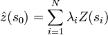
Using the information from the semivariogram an empirical model can be derived (Equation 3). The fitted semivariogram is used to determine the weights, λ_i, required for local interpolation. The weights are chosen so that the estimate, z(x₀), is unbiased and the estimation variance is less than it would be for any other linear combination of the input data.

Equation 3

$\hat{z}(x_0) = \sum_{i=1}^n \lambda_i \times z(x_i)$

where λ_i are the weights derived from the semivariogram.

This model (Equation 3) applies to ordinary, simple and universal kriging which differ in their assumptions about the mean: ordinary kriging assumes a constant, unknown mean; simple kriging assumes a constant, known mean; and universal kriging assumes a trending mean. Additionally, data are often available for more than one variable at the measured points. If the secondary variables are correlated with the primary variable being modelled (and are known at the unsampled locations) they may be used to help predict conditions at unsampled locations by co-kriging.

References

• Burrough, P. A. and McDonnell, R. A. 1998 Optimal interpolation using geostatistics. In: Principles of Geographical Information Systems (Burrough, P.A. and McDonnell, R.A. eds.), Oxford: Oxford University Press, 132-161.
• de Smith M., Goodchild H.F. and Longley P.A, 2009. Geospatial Analysis - a comprehensive guide. 3rd Edition. Issue version 3.11. (see chapter 6.6 and 6.7 under "Contents, figures and tables")
• ESRI 2001. ArcGIS Geostatistical Analyst: statistical tools for data exploration, modelling and advanced surface generation. An ESRI White Paper.

ESRI 2001 ArcGIS 9 Geostatistical Analyst Tutorial.

• ESRI. 2001, Using ArcGIS Geostatistical Analyst ESRI, Redlands, CA.
• Li, J. and Heap, A.D., 2008 A review of spatial interpolation methods for environmental scientists. Geoscience Australia, Record 2008/23, 137 pp.
• Tobler, R. 1979 Smooth pycnophylactic interpolation for geographical regions. Journal of the American Statistical Association 74 (367), 519.