Spatial resolution
- The text on this page is taken from an equivalent page of the IEHIAS-project.
Geographic variations in the environment and population of interest mean that assessments are greatly affected by the spatial scale (or more strictly ‘spatial resolution’) at which the analysis is done. They also need to be considered in selecting the way in which the results are displayed and communicated.
Results of most assessments are given in a relatively aggregated form (e.g. as total impacts for the whole study population). Analysis, however, is generally done at a more detailed level, in order to reflect the highly localised (and often individual-level) interactions that really occur between environment and human health.
Decisions about the spatial resolution for the analysis can have profound effects on the estimated impacts. In general, the coarser the resolution (i.e. the more aggregated the analysis), the more attenuated the estimates will become: extremes will be lost and the distribution of impacts will appear much narrower than it really is. As a consequence, local hot-spots or severely at-risk populations may be missed, while abrupt (and artificial) differences in impact may appear to exist between adjacent areas. How much this affects the overall estimate of impact (across the study population as a whole) will vary. If relationships between exposure and health are linear, the effect is likely to be small. Where the relationships are non-linear, however, carrying out the analysis at a coarse resolution can strongly bias the estimates. As the attached worked example illustrates, however, changing the resolution of the analysis can alter both the estimated levels of impact and their apparent spatial distribution.
Choosing an appropriate resolution needs care. We do not necessarily get better results simply by using a finer resolution (i.e. smaller study units), for two reasons. First, this may add to the uncertainty in our estimates of exposures, because we do not have reliable data at a local level. Secondly, it exacerbates the 'small number problem' in terms of estimates of risk, because each study unit contains only a few people. For rare effects, especially, the estimated impacts then become vanishingly small (e.g. with excess risks of only a fraction of a person in each area). This can make the results difficult to interpret, especially for non-specialist users.
The watchwords for choosing the spatial resolution should thus be:
- Select a resolution for analysis that reflects the scale of the phenomena being studied (e.g. the spatial variations in the hazards and the populations that might be affected);
- Select a resolution for display and communication of the results that:
- is no smaller (and preferably coarser) than that of the analysis;
- provides stable estimates of impact in each study unit;
- enables users to identify relevant variations in the impacts (e.g. local hotspots) that might merit attention.
Worked example
This example illustrates how results of an assessment can vary with spatial resolution of input data.
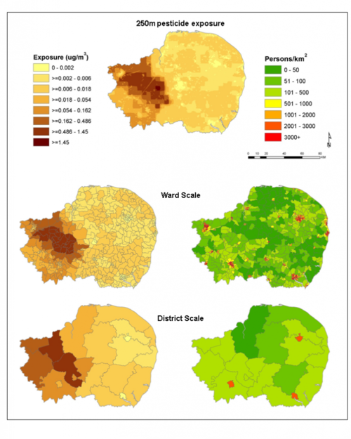
The exposure data are taken from an assessment of the potential health impact of pesticides, in the East Anglia region of Great Britain, in which ambient pesticide exposures were modelled for a 250x250m grid. The effect of spatial scale on the final estimate of health impact is illustrated.
GIS was used to area-weight the modelled exposures so they could be mapped at two additional scales: wards and district level. For comparison, a common classification (Table 1) was applied to the different exposure maps. The total population within each class was computed, from postcode headcount data, and exposure profiles derived (Figure 1). Figure 2 shows the mapped exposures and population densities for each spatial scale.
| Class | Exposure (µg/m3) |
|---|---|
| 1 | 0 - 0.002 |
| 2 | >= 0.002 - 0.006 |
| 3 | >= 0.006 - 0.018 |
| 4 | >= 0.018 - 0.054 |
| 5 | >= 0.054 - 0.162 |
| 6 | >= 0.162 - 0.486 |
| 7 | >= 0.486 - 1.45 |
| 8 | >= 1.45 |
Figure 1. Pesticide exposure and population density at different spatial scales
Figure 2. Pesticide exposure distribution at 250m, ward and district level
On the basis of the estimated exposures, the expected number of cases attributable to pesticide exposure for a hypothetical disease was calculated for the whole of East Anglia. The base prevalence for the hypothetical disease was assumed to be 15 per 100,000. The following formula for attributable burden was used:
AB = (RR – 1 / RR) * P * F
Where:
RR is the relative risk
P the base prevalence for the disease
F the fraction of the exposed population.
Two exposure scenarios are presented:
- The first scenario is for a binary exposure, in which classes 1+2 (< 0.006 µg/m3) are the non-exposed group and classes 3 and above (>= 0.006 µg/m3) represent the exposed. The RR for the exposed group is 1.09.
- The second scenario includes the same non-exposed group, plus three exposure categories based on concentration.
- Low exposure includes classes 3+4 (>= 0.006 - 0.054 µg/m3) with a RR of 1.09
- Medium exposure includes classes 5+6 (>= 0.054 - 0.486 µg/m3) with a RR of 1.12
- High exposure is classes 7+8 (>= 0.486 µg/m3) with a RR of 1.17.
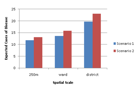
The results for these two scenarios for the different spatial scales are presented in Figure 3.
Figure 3. Expected cases of hypothetical disease due to pesticide exposure calculated at three spatial scales


