Spatial disaggregation
- The text on this page is taken from an equivalent page of the IEHIAS-project.
While statistical information on socio-economic activities is widely available, the data are often collected or released only at a relatively aggregated level. Census data, for example, are often aggregated to census tracts, in part because of concerns about confidentiality. Depending on their nature, data on economic activities may likewise be aggregated to country or regional administrative units. In the case of emissions, coarse grids may be used to reduce the data volumes and minimise the uncertainties inherent in more localised estimates.
In these aggregated forms, the data are useful for broad-scale assessments of health impacts, but using aggregated data has the danger of masking important local hotspots, and overall tends to smoothe out spatial variations in impact. As a result, it may also mean that crucial social inequalities in risk are overlooked. For this reason, assessments often need to disaggregate source data, in order to provide more localised estimates of potential exposures and to highlight effects of specific sources.
Spatial disaggregation or downscaling is the process by which information at a coarse spatial scale is translated to finer scales while maintaining consistency with the original dataset. Areal interpolation techniques can be used in this context to transform data from a set of source zones to a set of target zones with different geometry. Ranging in complexity from simple area weighting to dasymetric disaggregation, these approaches all have in common what Tobler termed the pycnophylactic, or mass-preserving, property in that the estimates are conditioned to sum to that of the source zones. These areal interpolation techniques are generally described below, using population as an example.
Contents
Simple area weighting
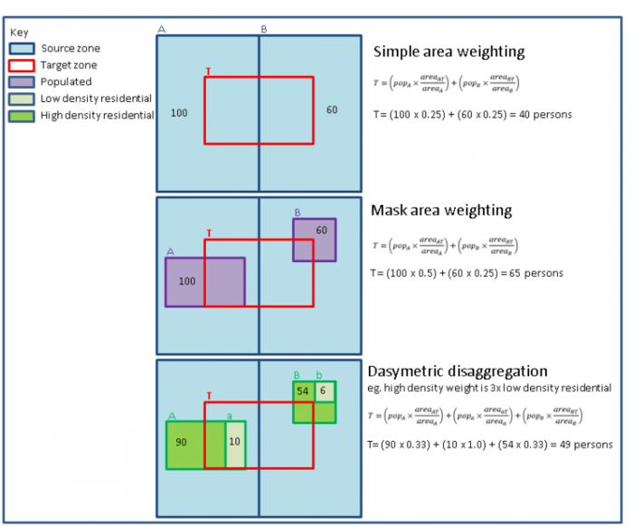
Mass-preserving areal interpolation (i.e. area-weighting) redistributes aggregated data based on the proportion of each source zone that overlaps with the target zone according to the following equation:
where: Pt is the population in target zone t; Ps is the population in source zone s; As is the area of source zone s; and Ats is the area of target zone t overlapping source zone s.
While area-weighting ensures that the total from the source data remains unchanged, it is based on the often incorrect assumption that the phenomena of interest are evenly distributed across the source zones. Population is one such example. Most populations, including that of the EU, are rarely uniform across census tracts, and instead tend to be highly clustered in urban centres surrounded by areas of dispersed rural homesteads.
Mask area weighting
Mask area weighting is an improvement on simple area weighting in that it uses a mask to define where, within the target zone, the source data should be allocated. This process is like binary dasymetric mapping, in which each source unit is divided into two sub-regions - populated and unpopulated – and the census information is then allocated only to the populated areas. Land cover can be used to identify populated areas and create the mask. The equation is as follows:
where: Atsp is the area of populated land that overlaps between the target map unit t and source map unit s; and Asp is the area of target map unit s that is populated land.
Dasymetric disaggregation
Dasymetric disaggregation is a type of areal interpolation that incorporates ancillary data to facilitate the areal interpolation process. It differs from choropleth mapping in that, rather than defining areas on the basis of administrative units, the boundaries derive from the actual spatial distribution of the variable being mapped. As mentioned in relation to mask area weighting, land cover data, in particular, offer a means by which residential areas can be distinguished from non-residential areas. Dasymetric disaggregation, however, is an improvement on mask area weighting in that two or more categories can be assigned weights for disaggregation. This is referred to as polycategorical dasymetric disaggregation. The challenge in dasymetric disaggregation thus involves devising an appropriate set of weights that can be applied to the land parcels (or other ancillary data) to reflect population density. Weights may be defined using selective sampling (see Stochastic allocation) or regression analysis.
Stochastic allocation
Gallego and Peedell (2001) and Gallego (2010) describe a stochastic allocation process by which weights are devised for disaggregating population totals from larger administrative units (NUTS 2 regions) to smaller ones (communes) on the basis of the land cover information. Communes were first stratified, by comparing the commune population density to the average density of the surrounding NUTS 2 region, into one of three levels reflecting population density (i.e. dense, less dense and no urban). The method then involved disaggregating the NUTS 2 totals using an initial set of weights, re-aggregating the population to the commune level and comparing it to the known total, computing a disagreement indicator, and adjusting the weights to reduce the disagreement. The iterative nature of this method involves effort in model tuning to achieve suitable weights. The result is a dasymetric population density grid for the European Union.


