Zone design
- The text on this page is taken from an equivalent page of the IEHIAS-project.
When spatial objects are analysed, the map area is usually portioned into zones. The definition of these zones involves the selection of the scale of the study and the aggregation of data to match the choice of scale. In nearly all cases, there are a large number of alternative scales and aggregations which could be used. It follows, therefore, that spatial data and the patterns and processes they describe are the product of a particular set of zonal boundaries, and that qualitative or quantitative studies of spatial data are not invariant with the choice of these boundaries. Therefore, scale and aggregation effects can be seen as fundamental characteristics of spatial data.
A number of important issues for map design and representation arise from this principle. One of these is the so-called modifiable areal unit problem (MAUP). Fotheringham and Wong (1991) define the MAUP as the sensitivity of (spatial) analytical results to the definition of units for which data are collected. It is a classical problem associated with the design and display of boundaries. As implied above, the modifiable areal unit problem has in reality two separate but interrelated aspects: scale (or more accurately, resolution) and zoning. The resolution issue is defined as “the variation in results that may be obtained when the same areal data are combined into sets of increasingly larger areal units of analysis” (Openshaw and Taylor, 1979; Openshaw, 1984). Wrigley et al. (1996) suggest that this effect is a tendency, within a system of modifiable areal units, for different statistical results to be obtained from the same set of data when the information is grouped at different levels of spatial resolutions. (For an example, see link to Worked example, below).
Scale differences are the most obvious manifestation of the modifiable areal unit problem but there is also the problem of alternative combinations of base units at equal or similar scales. Openshaw and Taylor (1979) define this issue as an aggregation (or zoning) problem: ‘any variations in results due to alternative units of analysis where n, the number of units, is constant’. Openshaw (1984) suggested that this aggregation problem can arise because of the way data are aggregated to form any given number of zones. In the aggregation problem, a map with a certain scale (n) can have infinitive possibilities to where areal units can be joined. He argued that the zoning effect is greater than the scale effect because there is more freedom to choose the delineation of boundaries than for choosing the numbers of zones are required (Openshaw, 1984).
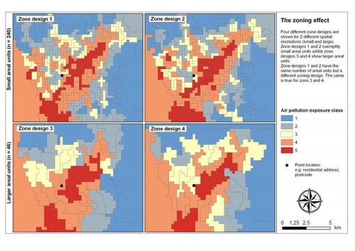
Figure 1, below, shows examples of the scale and zoning effects, using a simulated example developed in SIENA. The maps all show the same data (average exposure to air pollution, classified into quintiles). The two maps in each row have the same number of spatial units, but have units defined on the basis of different optimising rules (so have different boundaries). The maps in the upper row are based on small areal units; those on the lower row on larger areal units. Differences in the mapped distributions are evident, both between columns (zoning effect) and between rows (scale effect). It may easily be imagined that spatial patterns of other, related variables (e.g. disease rates) would also vary between the different zone designs. In this case, the spatial relationships between the two variables (e.g. air pollution exposure and health) would also vary, depending on which zone design was used.
This example highlights the importance of selecting the zone design used for mapping and analysis with care. It also suggests that some form f sensitivity analysis may often be useful, to determine how stable the spatial patterns in, and spatial relationships between, the variables really are.
References
- Fotheringham, A.S. and Wong, D. 1991 The modifiable areal unit problem in multivariate statistical analysis. Environment and Planning A 23, 1025-1044.
- Openshaw, S. and Taylor, P.J. 1979 A million or so correlation coefficients: three experiments on the modifiable areal unit problem. In: Statistical applications in the spatial sciences. (Wrigley, N., ed.),. London: Pion: London, pp 127-144.
- Openshaw, S. 1984 The modifiable areal unit problem (concepts and techniques in modern geography). Norwich: Geo Books, Norwich, p 41.
- Wrigley, N., Holt, T., Steel, D. and Tranmer, M. 1996 Analysing, modelling, and resolving the ecological fallacy. In: Spatial analysis: modelling in a GIS environment. (Longley, P. and Batty, M. eds.), Cambridge: Geoinformation International, pp 25-40.

